Mathematically, this time scale dichotomy results in problems with a distinct structure. The short time scale (instantaneous) state of channels is described by a random vector $\bbh$ whose different components represent the state of individual channels. When the system observes a channel realization $\bbh$ it allocates resources $\bbp(\bbh)$ that result in an instantaneous performance outcome $\bbf\big(\bbp(\bbh), \bbh\big)$. Both, the resources $\bbp(\bbh)$ and the performance outcomes $\bbf\big(\bbp(\bbh), \bbh\big)$ are vectors because we may have multiple channels, multiple resources to allocate in each channel, and multiple outcomes of interest for each channel.
The time scale dichotomy dictates that the instantaneous performance $\bbf\big(\bbp(\bbh), \bbh\big)$ is not experienced by the user whose (human) response time is much too slow. The performance experienced by the user is the average of instantaneous performances which, if we are operating under conditions where the law of large numbers holds, is given by the expectation
\begin{equation} \label{eqn_x}
\bbx =\mbE\big[\bbf\big(\bbp(\bbh), \bbh\big)\big].
\end{equation}
Our goal as wireless system designers is to optimize the average performance $\bbx$. Since this is a vector we introduce a utility $f_0(\bbx)$ and a set of constraints $\bbg(\bbx)\geq\bbzero$ and define the optimal resource allocation $\bbp^*(\bbh)$ as the one with maximum utility
\begin{align} \label{eqn_problem}
\max \ \ & f_0(\bbx) , \\ \nonumber
\text{s.t.}\quad & \bbx \leq \mbE\big[\bbf\big(\bbp(\bbh), \bbh\big)\big], \quad
\bbg(\bbx)\geq\bbzero.
\end{align}
where the equality in \eqref{eqn_x} is relaxed to an inequality to make the problem a little more tractable. This relaxation is without loss of optimality if the utility $f_0(\bbx)$ is nondecreasing.
As a simple example consider a point to point channel. The random variable $h$ is a scalar representing the instantaneous channel strength to which the system responds by allocating power $p(h)$. The received signal strength is the product $hp(h)$ and the communication rate achieved during the frame is $\log(1 + hp(h))$. It is of interest to maximize expected capacity $c = \mbE\big[ \log(1 + hp(h)) \big]$ subject to an average power constraint $p = \mbE\big[ p(h)\big]\geq p_0$. This problem is of the form in \eqref{eqn_problem} if we make the vector $\bbx=[c,-p]$, the utility $f_0(\bbx)=c$ and the constraint $g(\bbx) = p_0-p$.
In reality we are interested in more complicated problems in which there are multiple terminals with multiple channels sharing the same bandwidth and the rate functions are more complicated than the capacity-achieving logarithm. These problems can get very difficult to solve and there is a rich literature to find their solutions or their approximate solutions (see our paper for some concrete references.). The recent and growing success of learning methods raises the question of whether and how they are applicable to solve the resource allocation problem \eqref{eqn_problem}. Let us try to answer these questions.
Learning Optimal Resource Allocations
Although it may not look like it, the problem in \eqref{eqn_problem} has the structure of a statistical loss, which is the sort of problem to which machine learning techniques are applicable. If $\bbh$ is a feature vector, $\bbp(\bbh)$ is a regressor or classifier we want to learn, $\bbf\big(\bbp(\bbh), \bbh\big)$ is a loss function, and the expectation $\mbE\big[\bbf\big(\bbp(\bbh), \bbh\big)\big]$ is a statistical loss over the distribution of the feature vector. None of this is true since $\bbh$ is a fading realization, $\bbp(\bbh)$ a resource allocation, $\bbf\big(\bbp(\bbh), \bbh\big)$ an instantaneous communication performance metric, and $\mbE\big[\bbf\big(\bbp(\bbh), \bbh\big)\big]$ an average communication performance metric. But none of these differences are mathematically relevant.
Once we notice this mathematical equivalence, it is ready to consider the use of a parameterized model in which we write the resource allocation as $\bbp(\bbh) = \bbphi(\bbh,\bbtheta)$. Using this parameterization we rewrite \eqref{eqn_problem} as
\begin{align} \label{eqn_param_problem}
\max \ \ & f_0(\bbx) , \\ \nonumber
\text{s.t.}\quad & \bbx \leq \mbE\big[\bbf\big(\bbphi(\bbh,\bbtheta), \bbh\big)\big], \quad
\bbf(\bbx)\geq\bbzero,
\end{align}
where the optimization is over the parameter $\theta$ instead of the resource allocation $\bbp(\bbh)$. It is important to observe that the parameterization $\bbphi(\bbh,\bbtheta)$ restricts the form of the resource allocation in \eqref{eqn_param_problem}. Thus, \eqref{eqn_param_problem} is a good proxy for \eqref{eqn_problem} inasmuch as $\bbphi(\bbh,\bbtheta)$ allows for a good description of optimal resource allocations. For example, if we use a linear parameterization $\bbphi(\bbh,\bbtheta) = \bbtheta^T\bbh$ it’s unlikely that the solution of \eqref{eqn_param_problem} is a good approximation to the solution of \eqref{eqn_problem}. In our experiments, we use neural network parameterizations and observe that they work well. But little is known about appropriate learning parameterizations for wireless communications systems.
The problem in \eqref{eqn_param_problem} does has an important difference with conventional learning problem: The statistical loss appears as a constraint. One can think that this is a little bit of an artificial difference because we could replace $\bbx$ with $\mbE\big[\bbf\big(\bbphi(\bbh,\bbtheta), \bbh\big)\big]$ in the objective. But if we do that we also need to replace it in the constraint $\bbf(\bbx)\geq\bbzero$ and we end up again with a statistical loss constraint. In fact, the presence of constraints is a fundamental property of wireless systems as we are invariably trying to balance the competing rate, bandwidth and power requirements of different users. In order to handle the constrained statistical learning problem in \eqref{eqn_param_problem} we develop mechanisms for learning in the dual domain.
Learning in the dual domain
The fact that the parameterized learning problem we formulate in \eqref{eqn_param_problem} is constrained not only distinguishes it from classical regression problems or those that appear in reinforcement learning, but more importantly means that such existing gradient-based algorithms to solve cannot be applied directly to the learning formulation of the resource allocation problem. To apply such methods, it is then necessary to formulate an appropriate unconstrained problem. An immediate or natural approach for deriving an unconstrained problem is to add an additional term to the objective in \eqref{eqn_param_problem} that penalizes violations of the constraints. Maximizing such an objective will indeed strike some balance between maximizing $f_0(\bbx)$ and avoiding constraint violation, but will do so in a manner that is sub-optimal. What we seek is such a penalty-based reformulation whose solution is equivalent, or at least near-equivalent, to that of \eqref{eqn_param_problem}.
Those familiar with convex optimization may naturally consider the idea of Lagrangian duality. The so-called dual problem is a particular case of the penalty-based reformulation of constrained optimization problems, one which is widely known to have an equivalent solution when the original problem is convex (i.e., have convex objective and convex constraints). The dual problem is formulated as
\begin{align}\label{eqn_param_dual_function}
D^*_{\bbphi} := \min_{\bblambda, \bbmu} \max_{\bbtheta, \bbx} g_0(\bbx)+ \bbmu^T \bbg(\bbx)+ \bblambda^T \Big( \mbE\big[\bbf\big(\bbp(\bbh), \bbh\big)\big]- \bbx \Big),
\end{align}
where we introduce the nonnegative multiplier dual variables $\bblambda \in \reals_+^p$ and $\bbmu \in \reals_+^r$, associated with the constraints $\bbx\leq\mbE\big[\bbf\big(\bbp(\bbh), \bbh\big)\big]$ and $\bbg(\bbx)\leq\bbzero$ respectively.
We can think of \eqref{eqn_param_dual_function} as a penalized version of \eqref{eqn_param_problem} in which we also optimize over the penalty multipliers. This renders \eqref{eqn_param_dual_function} analogous to conventional learning objectives (albeit with a min-max structure) and, as such, a problem that we can solve with conventional learning algorithms. While it is known that the solution to dual problems are equivalent to that of their constrained counterparts when the original problem is convex, for general, potentially non-convex optimization problems, such as the one we consider in \eqref{eqn_problem}, this equivalence cannot be assumed. However, we can show that, in the case of sufficiently dense parameterizations (such as deep neural networks), the dual problem in \eqref{eqn_param_dual_function} is indeed near equivalent to that of the original resource allocation problem in \eqref{eqn_problem}—see Theorem 1 in our later referenced paper for details on this result.
A natural algorithm to perform on the min-max problem in \eqref{eqn_param_dual_function} is to sequentially update both the primal and dual variables over an iteration index $k$. We ascend and descend on the learning parameter $\bbtheta$ and dual variable $\bblambda$, respectively, with the following stochastic gradient descent updates
\begin{align}
\bbtheta_{k+1} &= \bbtheta_k + \gamma_{\bbtheta,k} \widehat{\nabla_{\bbtheta}}\mathbb{E}_{\bbh} \bbf(\bbphi(\bbh,\bbtheta_{k}),\bbh) \bblambda_k , \label{eq_spd_update1} \\
\bblambda_{k+1} &= \left[ \bblambda_k – \gamma_{\bblambda,k} \left( \hbf(\bbphi(\hbh_k,\bbtheta_{k+1}),\hbh_k) -\bbx_{k+1} \right) \right]_+\label{eq_spd_update3}.
\end{align}
We can likewise perform similar ascent/descent updates on $\bbx$ and $\bbmu$. The updates in \eqref{eq_spd_update1}-\eqref{eq_spd_update3} are notable in that they employ stochastic—or model-free—estimates the gradients of \eqref{eqn_param_dual_function}. We say they are model-free because they can be computed without explicit knowledge of the functions in \eqref{eqn_problem}, e.g., without knowing $\mathbb{E}_{\bbh} \bbf$. Popular model-free gradient estimates include, for example, the finite difference method or policy gradient method, each of which only require the ability to sample function values at given points. Thus, by converting to the dual domain with dense function parameterizations, we acquire a near-equivalent unconstrained problem in \eqref{eqn_param_dual_function} with a natural, model-free learning algorithm in \eqref{eq_spd_update1}-\eqref{eq_spd_update3}.
Deep Neural Networks
As briefly mentioned in the previous section, the near-equivalence of the unconstrained dual problem rests on a notion of denseness, or in other words universality, of the parameterization $\bbphi(\bbh,\bbtheta)$ of the resource allocation function $\bbp(\bbh)$. This is to say that we wish to consider parameterizations that have the ability to approximate arbitrary functions well. While there are numerous well-known parameterizations that fit this description, from polynomial expansions to reproducing kernel Hilbert space expansions, one popular learning model that fits this universality condition is the deep neural network (DNN). DNNs are not only theoretically known to be universal function approximators, but have been shown in extensive empirical evaluation to have strong generalization abilities. Moreoever, very simple stochastic gradient methods such as the one in \eqref{eq_spd_update1}-\eqref{eq_spd_update3} are observed to find good solutions in NN problems, despite the non-convexity of the DNN model.
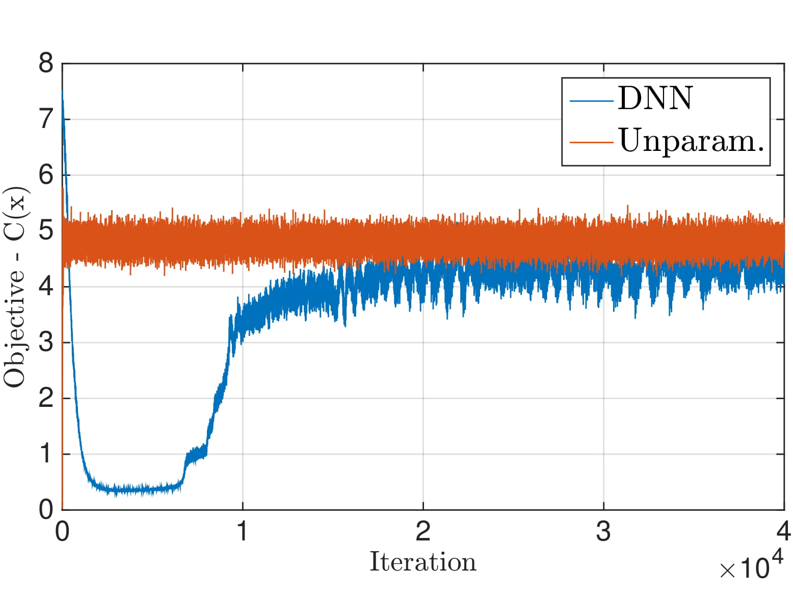
We can then use a DNN to parameterize the resource allocation function, and perform the stochastic learning method to find the best parameter $\bbtheta$—which here denotes the inter-layer edge weights of the DNN—to approximate the optimal resource allocation function. As a simple demonstration of this approach, consider the problem of allocating transmission power across $m$ transmitters so that we may maximize the aggregate capacity achieved across all transmitters subject to a shared power budget constraint. If we ignore any inter-user interference, an exact solution to the problem can be found without any of the learning parameterizations discussed here. This is nonetheless an instructive example, as it gives us a baseline with which to compare the solutions found via our proposed learning method. In the figure below, we the performance obtained by the exact, unparameterized solution and that obtained by a DNN parameterization using the proposed learning algorithm. We observe that, after the training process has converged, we have obtained similar performance using a DNN, all without any explicit model knowledge of the system.
To Learn Or Not To Learn
Throughout this post we have discussed the use of learning techniques in the solution of optimal resource allocation problems in wireless communications. There are four important conclusions that bear emphasizing:
Optimal resource allocation problems in wireless systems are closer to statistical machine learning than one would expect a priori. The sole difference is that wireless communication systems lead to formulations in which a statistical loss naturally appears as a constraint, whereas in conventional machine learning problems the statistical loss appear in the objective.
To handle constraints we formulate learning in the dual domain. We do that with a primal-dual stochastic optimization algorithm that seeks convergence to a saddle point of the Lagrangian function.
Learning in the dual domain carries no loss of optimality if we use universal parameterizations. If we are able to find Lagrangian minimizers we are guaranteed to find the optimal resource allocation because there is no duality gap despite the lack of convexity in the resource allocation function. The Lagrangian can be difficult to minimize because it is not convex, but this is the same challenge that arises when minimizing a nonconvex statistical loss. There is no further optimality penalty for working on the dual domain.
Learning methods are model-free. We can learn an optimal resource allocation without ever having access to the channel distribution or to the form of the functions that map resource allocations to instantaneous performance metrics.
The points above show that we can use learning techniques for optimal wireless system design. However, they do not provide an answer to the question of whether we should. At this point, we can’t provide a definitive answer but there are two reasons why the question is at least worth asking. The first reason is that resource allocation problems in wireless communications have resisted efforts to develop optimal solutions. We know how to solve some specific instances of \eqref{eqn_problem} but there are many other ones in which we don’t know how to find optimal solutions. In these instances we develop heuristics and there really is no reason why they should not be outperformed by a learned solution. In fact, we can think of learning as a way of devising heuristics. Just one in which the heuristic is data-driven instead of designer-driven.
A second, perhaps stronger, argument is that models are not necessarily known and certainly not perfect. Solving resource allocation problems necessitates knowledge of the functions that map resource allocation to rates as well as knowledge of the channel distribution. Problems with these assumption can arise in pretty simple scenarios. For instance, in point to point channels the instantaneous rate function $\log(1 + hp(h))$ is, in practice, replaced by a collection of modes that are chosen adaptively. These modes are combinations of codes and modulation schemes that support a certain communication rate and we choose a code and a power allocation that we think would result in successful packet delivery. We can model this strategy by defining a function $c(h,p(h))$ whose value is the rate attained by the mode chosen for channel realization $h$ and power allocation $p(h)$. This still leads to formulations like \eqref{eqn_problem} with $c = \mbE\big[ c(h,p(h)) \big]$. However, the rate $c(h,p(h))$ is not something we know for certain. Uncertainties in channel estimation and interference environments lead to lost packets and differences between the expected rate predicted by the model $c(h,p(h))$ and the actual rate attained in practice. A learned resource allocation would not suffer degradation from this mismatch between model and reality because it does not rely on a model. Granted, in the case of a point to point channel there is likely no need to resort to learning techniques to overcome a simple model mismatch. But in reality we are interested in more complex systems with multiple terminals and competing goals where the effects of model mismatch need not be as straightforward.
To Read Further
Source: M. Eisen, C. Zhang, L. Chamon, D. Lee, and A. Ribeiro ”Learning Optimal Resource Allocations in Wireless Systems.” IEEE Transactions on Signal Processing. August 2018 (submitted).
Points of Contact: Mark Eisen and Alejandro Ribeiro.